Tutorial Aims:
1. Understand why you should use R to make study maps.
2. Learn how to convert UK National Grid References into Longitude and Latitude.
3. Learn how to make local and global (interactive) study maps with leaflet.
4. Learn how to beautify your study maps.
Steps:
1. Import and check data
2. Convert UK National Grid References into Longitude and Latitude
3. Make small-scale study maps for study sites in Edinburgh
4. Make global-scale study maps (using clustering)
5. Challenge yourself!
In this Tutorial we will learn how to make beautiful and informative study maps using the package leaflet.
Why use R to make study maps?
In Ecology, we often conduct studies in the field at many different sites. Having a study map of all your different sites is good practice and helps anyone reading your research to put it into context. The coordinates in the Edinburgh dataset were collected during a university field course I went on in September of this year. We were measuring invertebrate abundance along public footpaths in Edinburgh to assess disturbance levels. When it came to writing up the field trip report, I did what I always do. I added the coordinates manually as pins on Google Maps and took a screenshot. How unscientific I hear you say! And you are right, why not use R to make study maps that first of all look better and don’t take much longer to create!
In this tutorial we will look at some ways of creating study maps in R, to create informative, accurate and beautiful maps for any study we want, be it small and local or global. Here, I will focus on the leaflet package, an open-source Java script library that allows us to create informative and even interactive maps! JAVA SCRIPT, I thought we were coding in R??? Don’t worry, you don’t need to know Java script in order to use the leaflet package!
A problem I have often come across when conducting fieldwork in the UK, is the different ways to note down coordinates. In the UK, we often use grid references based on the Ordnance Survey National Grid Reference system. This gives coordinates as Eastings and Northings rather than Longitude and Latitude. For most mapping packages you need to have your coordinates in Longitude and Latitude, so the first part of the tutorial will be on how to transform coordinates.
Getting started
This tutorial is primarily aimed at second or third year Ecology students (but I am in fourth year and only just learnt how to make study maps in R!). However, the skills you learn in this tutorial are widely applicable to other fields, so if you are not an ecologist still read on!
To complete this tutorial, you should have some prior knowledge of R. Check out this Intro to R Tutorial if you are new to R. You will also need some basic data manipulation skills in order to get the data into the format in which we can plot it with leaflet.
All materials you need for this tutorial can be downloaded from this GitHub repository. Clone and download the repo as a zip file, then unzip it.
1. Import and check data
Open R studio, start a new script and give it an informative name (e.g. leaflet_tutorial.R). Add some informative comments at the top of your script, for example the title of the tutorial, your name, and the data. Set your working directory to where the folder you just downloaded is. Load the packages we will need for the tutorial. If you have not installed any of them before use install.packages("package name") before loading them with the library function.
You can copy and paste the code chunks as you go through the tutorial.
# Set the working directory
setwd("your_filepath")

# Libraries ----
library(tidyverse)   # Data manipulation
library(leaflet)     # Interactive mapping
library(sf)          # Working with spatial data (converting coordinates)
library(mapview)     # Saving static maps
library(htmlwidgets) # Saving dynamic maps as htmls
Let’s load the data file containing the locations for some field work I did in Edinburgh recently:
# Load data
edi <- read.csv("edi_coords.csv")

# Explore data
head(edi)
str(edi)
Exploring the data shows that there are two sites: Craigmillar and Blackford, with seven transects each. We also notice that the coordinates are not in the conventional Longitude Latitude format! leaflet requires coordinates in this format though! What to do?!
2. Convert UK National Grid References into Longitude and Latitude
Don’t panic, we can convert UK grid references into Longitude and Latitude in R! This will involve some data wrangling and some useful functions from the sf package. sf stands for simple features and the package is used for processing spatial data. I won’t go into the details here, but sf objects are essentially data frames, which means they are tidy friendly (we can use functions form the tidyverse to manipulate them). Here, we use some functions from the sf package to convert Eastings and Northings in our edi dataset into Longitude and Latitude.
# Transform Easting and Northing from BNG into Longitude and Latitude
edi_coords <- edi %>%  # making new data frame called edi_coords
  st_as_sf(coords = c("Easting", "Northing"), crs = 27700) %>%
  # This function converts a foreign object to an sf object
  # Here, it transforms the object "edi"
  # The two columns "Easting" and "Northing" are identified as containing the coordinates
  # crs stands for coordinate reference system and is set to the UK
  st_transform(4326) %>%
    # This function transforms the sf object we just created from BNG to long and lat
  st_coordinates() %>%  # this function retrieves the new long lat coordinates into a matrix
  as_tibble()           # and matrix is transformed into a tibble (a simple data frame)
Did you know that st in the functions from the sf package stands for ‘spatial’ and ‘temporal’??
Now we have a tibble with all the Longitudes and Latitudes for our study sites. We now need to combine these with our original dataset:
# Combine our new coordinates with original data frame into a new data frame
edi_sites <- cbind(edi,edi_coords)  # now have long and lat in same dataset

# You might notice that our columns containing Long and Lat are called X and Y at the moment
# This is not very informative, so we will rename them:

# Rename columns X and Y to more informative names
edi_sites <- edi_sites %>%
  rename(Longitude = X, Latitude = Y)
Now we are ready to start mapping!
3. Make small-scale study maps for study sites in Edinburgh
As I said in the introduction, the Edinburgh dataset is from a University field course I went on. It was only a four day study and as such we only sampled two sites. We will first map all transects at both sites in one map and then zoom in to each site.
Edinburgh-wide Map
# Time to use the `leaflet` package!
(edi_map_pin <- leaflet(data = edi_sites) %>%  # Creating a leaflet object
    addTiles() %>%                             # Adding default OpenStreetMap background
    addMarkers(lng = ~ Longitude,              # Adding markers for study sites
               lat = ~ Latitude) %>%
    addScaleBar(position = 'bottomleft'))      # Adding scale bar
‘Voila’, just like that we have made our first study map with leaflet!
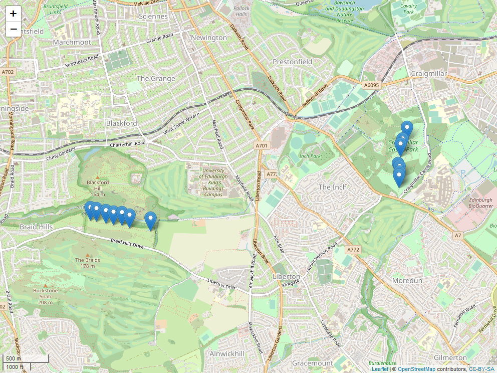
Locations of transects at the two sites: Craigmillar Castle Park and Blackford Hill.
Now, this map is may not be the prettiest. However, we are by no means finished yet. We can change the pin markers to many other forms, let’s try points instead:
# Map with points instead of pins
(edi_map_point <- leaflet(data = edi_sites) %>%  # Creating a leaflet object
    addTiles() %>%                               # Adding default OpenStreetMap background
    addCircles(lng = ~ Longitude,                # Adding markers for study sites
               lat = ~ Latitude) %>%
    addScaleBar(position = 'bottomleft'))        # Adding scale bar
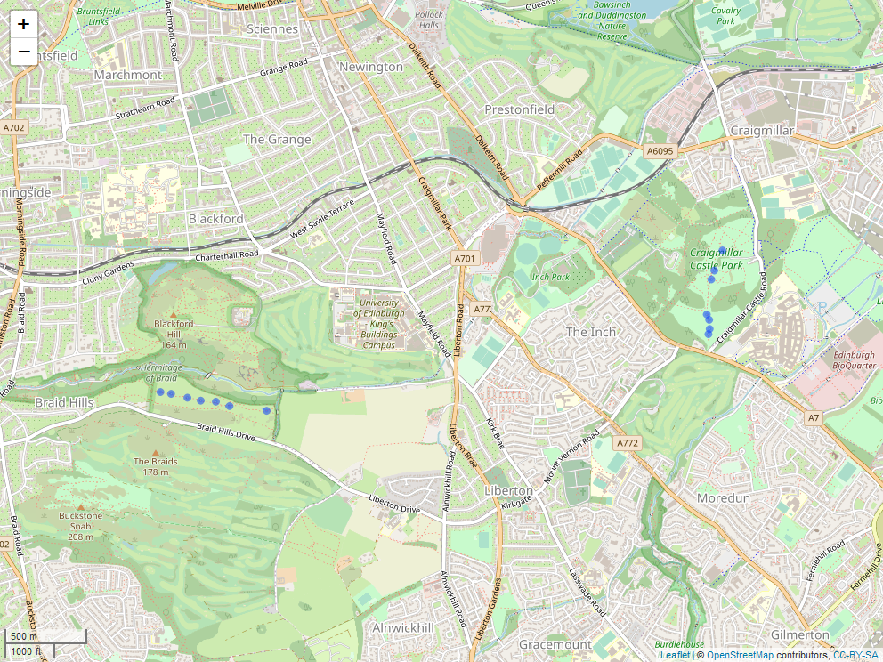
Locations of transects at the two sites: Craigmillar Castle Park and Blackford Hill.
That looks better already! Since we are plotting transects at both sites simultaneously the map is quite zoomed out and we don’t have a great level of detail. Here, it might make sense to map seperate maps for the two sites.
# Make two subset data frames:

craigm <- edi_sites %>%
  filter(Site == "Craigmillar")

blackf <- edi_sites %>%
  filter(Site == "Blackford")
Craigmillar Map
# Plot Craigmillar site
(craigm_map <- leaflet(data = craigm) %>%  # creating a leaflet object
    addTiles() %>%                         # adding default OpenStreetMap background
   setView(lng = -3.142849,                # Set coordinates for map centre
           lat = 55.92492,
           zoom = 15) %>%                  # Set zoom level
    addCircles(lng = ~ Longitude,          # Adding markers for study sites
               lat = ~ Latitude) %>%
    addScaleBar(position = 'bottomleft'))  # Adding scale bar
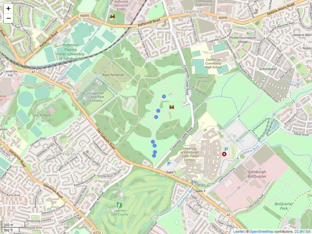
A study map for Craigmillar Castle Park, showing exact locations of the seven transects.
Blackford Map
# Plot Blackford site
(blackf_map <- leaflet(data = blackf) %>%  # creating a leaflet object
    addTiles() %>%                         # adding default OpenStreetMap background
   setView(lng = -3.190625,                # Set coordinates for map centre
           lat = 55.91831,
           zoom = 15) %>%                  # Set zoom level
    addCircles(lng = ~ Longitude,          # Adding markers for study sites
               lat = ~ Latitude) %>%
    addScaleBar(position = 'bottomleft'))  # Adding scale bar
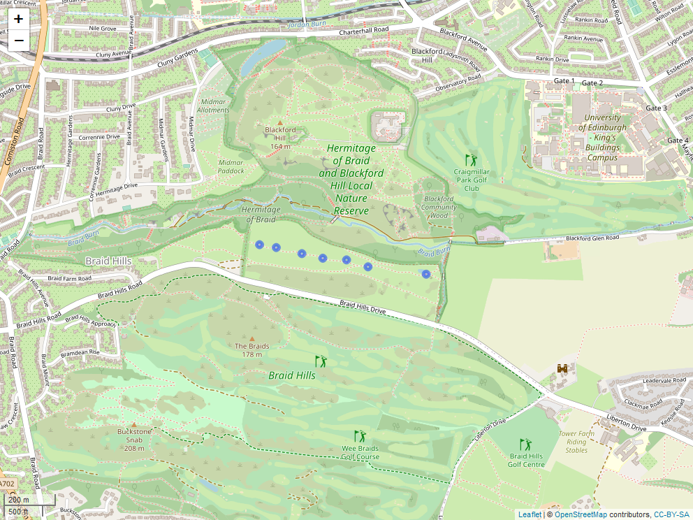
A study map for the Blackford Site, showing exact locations of the seven transects.
That looks much better than our first map! But we can do even more with leaflet. Let’s take the Blackford map and beautify it and add some informative interactive features.
# Add labels and change size of circles
(blackf_map2 <- leaflet(data = blackf) %>%
    addTiles() %>%                     # by default: Open Street Maps used
    setView(lng = -3.190625,           # Set coordinates for map centre
            lat = 55.91831,
            zoom = 15) %>%             # Set zoom level
    addCircleMarkers(lng = ~ Longitude,
                     lat = ~ Latitude,
                     label = ~ paste("Transect:", Transect),  # Label with transect number
                     radius = 2) %>%  # make circles smaller
    addScaleBar(position = 'bottomleft'))
Now if you hover your mouse over one of the circles in your plot viewer, a label with the transect number appears! By default this appears only when you hover the mouse over the marker. If you want the label to be always displayed, you have to include the labelOptions argument within the addMarkers (or addCircleMarkers in our case) function to set noHide to true.
Exporting maps
We have now created both static and dynamic study maps. If we wanted to include these maps in our report, send them to our parents to admire or publish them in our blog, we need to export them. We are using the function mapshot() from the mapview package to save static maps as png files, and the function saveWidget from the htmlwidgets package to save dynamic maps in html format.
# We have already loaded the two packages
# If you haven't used mapshot() before, you might need to install PhantomJS
# If that is the case, uncomment the following two lines:
# library(webshot)
# webshot::install_phantomjs()

# Save the Craigmillar map as a png
mapshot(craigm_map, file = "craigmillar_map.png", remove_controls = NULL)

# Save the interactive Blackford map in html format
saveWidget(blackf_map2, file = "blackford_map.html")
NB: The remove_controls argument set to NULLin the mapshot() function, ensures that the scale bar isn’t removed when we save the map!
If you want to save any of the other maps we have made so far, all you have to do is change the file names in the code above.
4. Make global-scale study maps (using clustering)
Now we have learnt how to make a local study map, suitable for ecological fieldwork on a small scale. What about large scale global studies though? Making a global map of study sites is just as easy, and there are some excellent interactive features within the leaflet package that we can use to visualise large numbers of sites.
For this part we will use data from the Reef Life Survey, a citizen science project which originated in Australia and conducts visual reef surveys all around the world (e.g. monitoring fish and invertebrate numbers). All their data is publicly available here. We will only use the dataset that contains the locations of all their study sites around the world.
# Load RSL survey locations data
rls_global <- read.csv("data/RLS_locations.csv")

# Simplify the dataset:
# Only keep long, lat and country name and rename columns to keep it consistent
rls_coords <- rls_global %>%
  select("CountryRegion", "SiteLatitude", "SiteLongitude") %>%
  rename(Latitude = SiteLatitude, Longitude = SiteLongitude, Country = CountryRegion)
Let’s plot all the survey locations around the world as points:
# Basic map with points for sites
(rls_map_point <- leaflet(data = rls_coords) %>%
    addTiles() %>%
    setView(lng = 0, lat = 30, zoom = 1) %>%
    addCircleMarkers(radius = 1) %>%
    addScaleBar(position = "bottomleft"))

# Save the map
mapshot(rls_map_point, file = "rls_map_point.png")
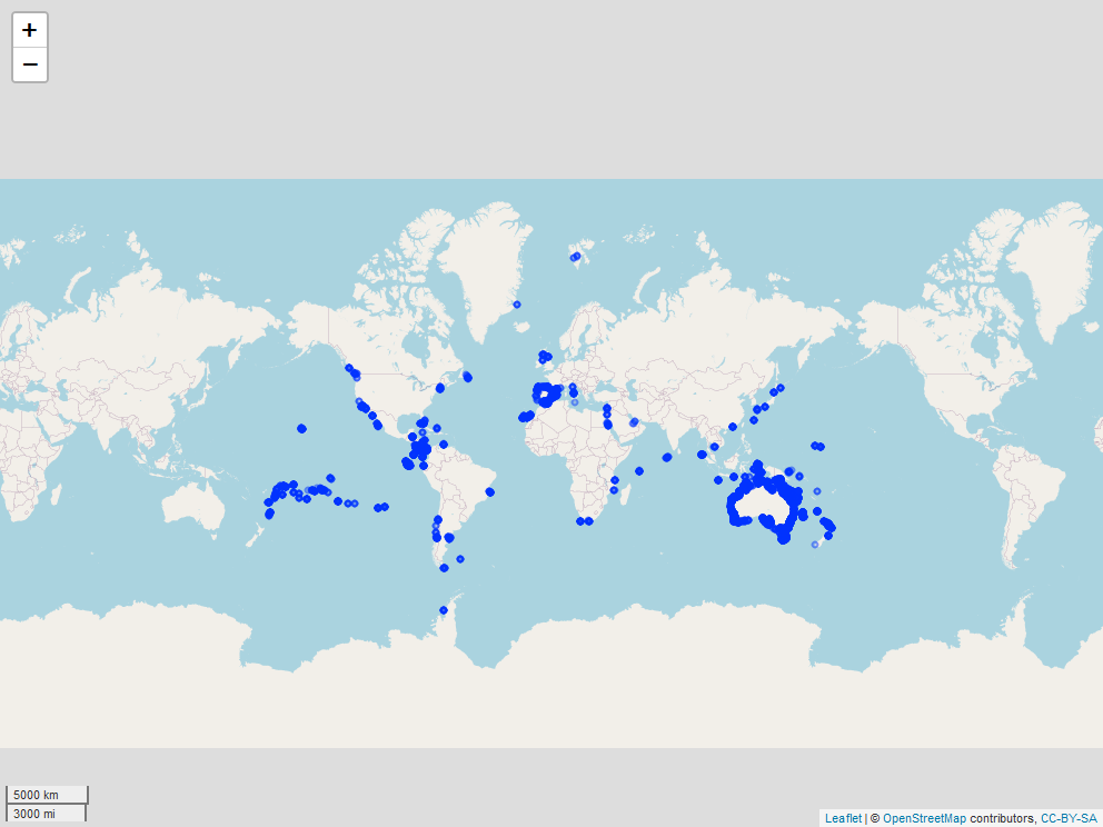
Locations of study sites of the Reef Life Survey globally
From this map we can see that the survey sites are all around the world! The highest concentrations of sites seem to be in Australia and Latin America. Again, we can make the map interactive by adding some more information. For example, the code below adds popups for the country names.
# Adding country popups
(rls_map_point_popup <- leaflet(data = rls_coords) %>%
    addTiles() %>%
    setView(lng = 0, lat = 30, zoom = 1) %>%
    addCircleMarkers(radius = 1,
                     popup = ~ Country) %>%  # Adding popups with country names
    addScaleBar(position = "bottomleft"))
Locations of study sites of the Reef Life Survey globally with country names as popup
Still, individual sites are quite hard to distinguish at this scale and with such a high number of points!
Luckily there is a very handy function in the leaflet package that we can use to cluster the sites! This means we group together sites in the same area in an interactive map. When you click on one cluster, the map zooms in and the cluster is split further into subregions. But see for yourself:
# Cluster survey sites
(rls_global_map <- leaflet(data = rls_coords) %>%
    addTiles() %>%
    setView(lng = 0, lat = 30, zoom = 1) %>%
    addMarkers(clusterOptions = markerClusterOptions()) %>%  # This line clusters our sites
    addScaleBar(position = 'bottomleft'))

# Save as static and dynamic map
mapshot(rls_global_map, file = "outputs/rls_global_map.png")
saveWidget(rls_global_map, file = "rls_global_map.html")
Locations of study sites of the Reef Life Survey globally (clustered!)
One more thing we will do with our map is change the base map. leaflet automatically sets the basemap to OpenStreetMap with the add_Tiles() function. By replacing this function with addProviderTiles(""), we can change the background map style. Check out this website to browse for lots of different map styles! In the example below I chose a black and white theme, which I thought looked cool:
# Change the map style
(rls_global_map_dark <- leaflet(data = rls_coords) %>%
    addProviderTiles("Stamen.TonerBackground") %>%  # Changing the base map, insert any theme you like!
    addMarkers(clusterOptions = markerClusterOptions()) %>%
    addScaleBar(position = 'bottomleft'))

# Saving black and white map
mapshot(rls_global_map_dark, file = "outputs/rls_global_map_dark.png")
saveWidget(rls_global_map_dark, file = "rls_global_map_dark.html")
Locations of study sites of the Reef Life Survey globally (clustered!)
Still here? Well done! You have made to the end of the tutorial! Today you have learnt:
- How to convert coordinates so we can work with them in R
- How to create small-scale study maps and how to make them interactive
- How to create global-scale study maps, using clustering
5. Challenge yourself!
Now it’s your turn! Time to use your newly gained skills.
Have a look at the Edinburgh dataset. There are some columns we have ignored so far, e.g. elevation.
- Try to make an interactive map for Craigmillar and add a label or popup displaying the elevation at each transect (Hint: check out the second Blackford map if you are stuck).
- Now change the code so that the label is always displayed, not just when you hover the mouse on it.
You have recently collected some data in the field yourself? Perfect! Try to plot your study sites using leaflet!
Have a look at this leaflet cheat sheet for some useful tips and tricks.